A Tour of the flatsurf Suite#
The flatsurf software suite is a collection of mathematical software libraries to study translation surfaces and related objects.
The SageMath library sage-flatsurf provides the most convenient interface to the flatsurf suite. Here, we showcase some of its major features.
Defining Surfaces#
Many surfaces that have been studied in the literature are readily available in sage-flatsurf.
You can find predefined translation surfaces in the collection translation_surfaces.
from flatsurf import translation_surfaces
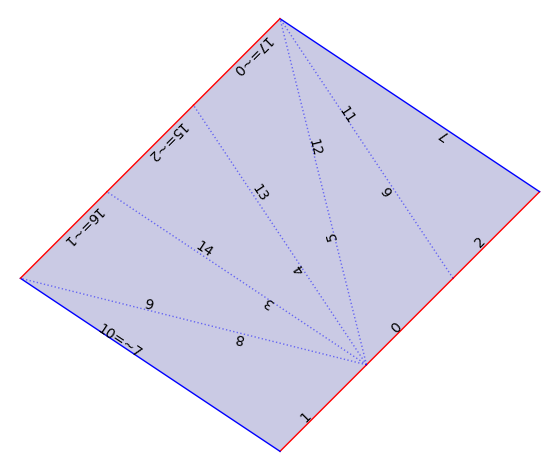
S = translation_surfaces.cathedral(1, 2)
S.plot()
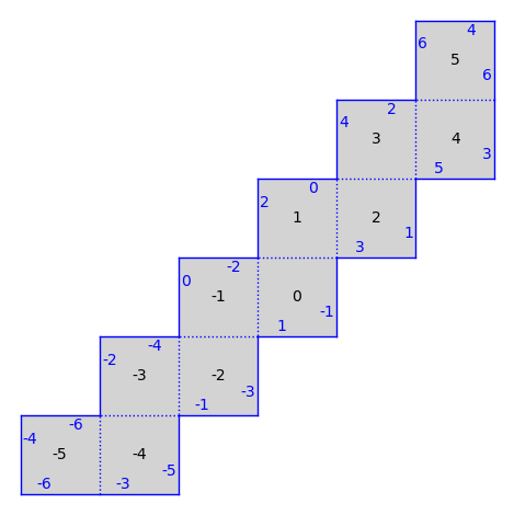
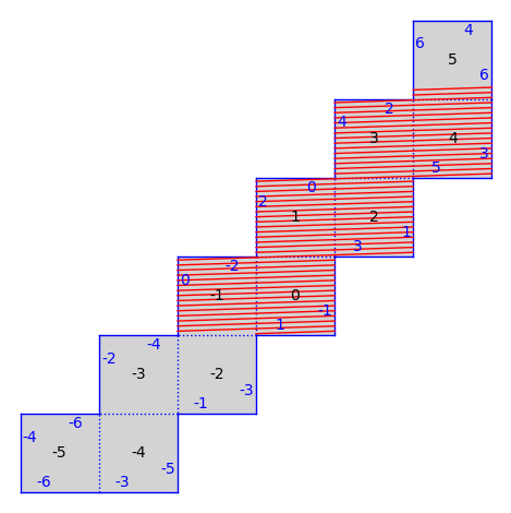
There are also infinite type surfaces (built from an infinite number of polygons) in that collection.
from flatsurf import translation_surfaces

S = translation_surfaces.infinite_staircase()
S.plot()
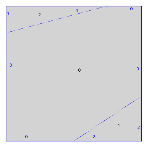
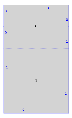
Some more general surfaces where the gluings are dilations are defined in the collection dilation_surfaces.
from flatsurf import dilation_surfaces

S = dilation_surfaces.genus_two_square(1/2, 1/3, 1/4, 1/5)
S.plot()
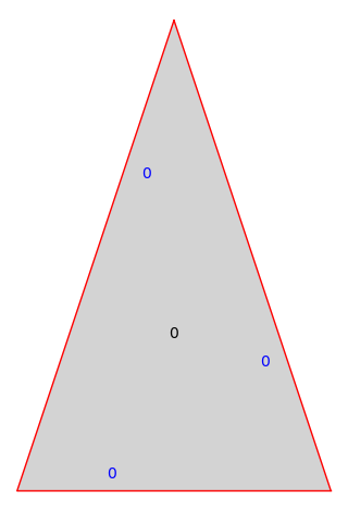
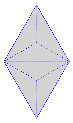
Even more generality can be found in the collection similarity_surfaces.
from flatsurf import Polygon, similarity_surfaces

P = Polygon(edges=[(2, 0), (-1, 3), (-1, -3)])
S = similarity_surfaces.self_glued_polygon(P)
S.plot()
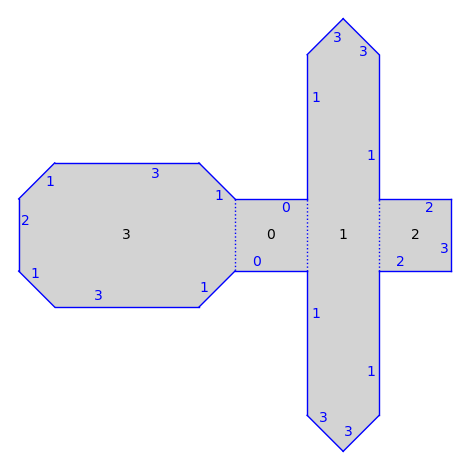
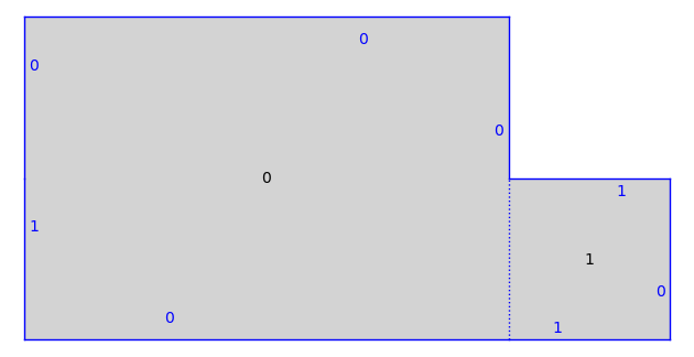
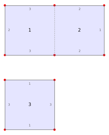
Building Surfaces from Polygons#
Surfaces can also be built from scratch by specifying a (finite) set of polygons and gluings between the sides of the polygons.
Once you call set_immutable(), the type of the surface is determined, here a translation surface:
from flatsurf import MutableOrientedSimilaritySurface, Polygon

hexagon = Polygon(vertices=((0, 0), (3, 0), (3, 1), (3, 2), (0, 2), (0, 1)))

square = Polygon(vertices=((0, 0), (1, 0), (1, 1), (0, 1)))

S = MutableOrientedSimilaritySurface(QQ)
S.add_polygon(hexagon)
S.add_polygon(square)

S.glue((0, 0), (0, 3))
S.glue((0, 1), (1, 3))
S.glue((0, 2), (0, 4))
S.glue((0, 5), (1, 1))
S.glue((1, 0), (1, 2))
S.set_immutable()

print(S)
S.plot()
Translation Surface in H_2(2) built from a square and a rectangle
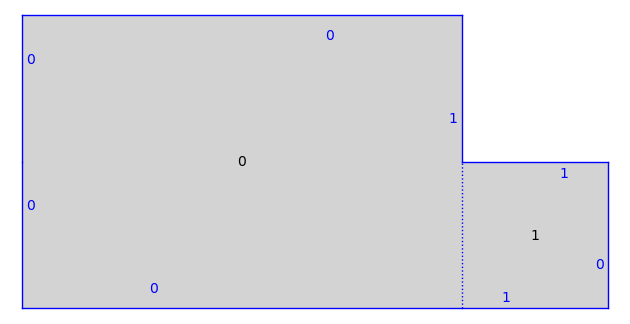
We can also create a half-translation surface:
T = MutableOrientedSimilaritySurface.from_surface(S)

T.glue((1, 1), (0, 2))
T.glue((0, 4), (0, 5))
T.set_immutable()

print(T)
T.plot()
Half-Translation Surface in Q_1(2, -1^2) built from a square and a rectangle
Or anything that can be built by gluing with similarities…
T = MutableOrientedSimilaritySurface.from_surface(S)

T.glue((0, 0), (1, 1))
T.glue((0, 5), (0, 3))
T.set_immutable()

print(T)
T.plot()
Genus 2 Surface built from a square and a rectangle
There is a relatively small contract that a surface needs to implement, things such as “what is on the other side of this edge?”, “is this surface compact?”, … so it is not too hard to implement infinite type surfaces from scratch.
Further Reading#
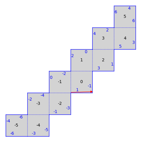
Trajectories & Saddle Connections#
Starting from a tangent vector, we can shoot a trajectory along that tangent vector. The trajectory will stop when it hits a singularity of the surface or after some (combinatorial) limit has been reached.
from flatsurf import translation_surfaces

S = translation_surfaces.infinite_staircase()
T = S.tangent_vector(0, (1/47, 1/49), v=(1, 1/31))

S.plot() + T.plot(color="red")
trajectory = T.straight_line_trajectory()
trajectory.flow(100)

S.plot() + trajectory.plot(color="red")
Note that on a finite type surface, we can compute a FlowDecomposition (see below) to determine how a surface decomposes in a direction into areas with periodic and dense trajectories.
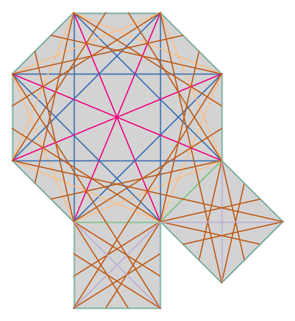
We can also determine all the saddle connections up to a certain length bound (on finite type surfaces).
from flatsurf import translation_surfaces
S = translation_surfaces.octagon_and_squares()

connections = S.saddle_connections(squared_length_bound=50)

# To get a more interesting picture, we color the saddle connections according to their length.
lengths = sorted(set(c.length() for c in connections))
color = lambda connection: colormaps.Accent(lengths.index(connection.length()) / len(lengths))[:3]

S.plot(polygon_labels=False, edge_labels=False) + sum(sc.plot(color=color(sc)) for sc in connections)
Further Reading#
Supported Base Rings#
Surfaces can be defined over most exact subrings of the reals from SageMath.
Here is an example defined over a number field:
from flatsurf import similarity_surfaces, Polygon

P = Polygon(angles=(1, 1, 4), vertices=[(0, 0), (1, 0)])
S = similarity_surfaces.billiard(P).minimal_cover(cover_type="translation")

print(S.base_ring())
S.plot(polygon_labels=False, edge_labels=False)
Number Field in c with defining polynomial x^2 - 3 with c = 1.732050807568878?
Here is a surface with a transcendental coordinate, supported through exact-real.
from pyexactreal import ExactReals

R = ExactReals(QuadraticField(3))
almost_one = R.random_element(1)

almost_one
/home/runner/work/sage-flatsurf/sage-flatsurf/.pixi/envs/doc/lib/python3.12/site-packages/cppyy/__init__.py:341: DeprecationWarning: pkg_resources is deprecated as an API. See https://setuptools.pypa.io/en/latest/pkg_resources.html
  import pkg_resources as pr
ℝ(1=2305843009213694107p-61 + ℝ(0.303644…)p-64)
from flatsurf import similarity_surfaces, Polygon

P = Polygon(angles=(1, 1, 4), vertices=[(0, 0), (almost_one, 0)])
S = similarity_surfaces.billiard(P).minimal_cover(cover_type="translation")

print(S.base_ring())
S.plot(polygon_labels=False, edge_labels=False)
Real Numbers as (Real Embedded Number Field in a with defining polynomial x^2 - 3 with a = 1.732050807568878?)-Module
Flow Decompositions#
We compute flow decompositions on the unfolding of the (2, 2, 5) triangle. We pick some direction coming from a saddle connection and decompose the surface into cylinders and minimal components in that direction.
from flatsurf import similarity_surfaces, Polygon
P = Polygon(angles=(2, 2, 5))
S = similarity_surfaces.billiard(P).minimal_cover(cover_type="translation")

G = S.graphical_surface(polygon_labels=False, edge_labels=False)
connection = next(iter(S.saddle_connections(squared_length_bound=4)))

G.plot() + connection.plot(color="red")
from flatsurf import GL2ROrbitClosure

O = GL2ROrbitClosure(S)
decomposition = O.decomposition(connection.holonomy())

decomposition
FlowDecomposition with 4 cylinders, 0 minimal components and 0 undetermined components
In this direction, the surface decomposes into 4 cylinders. Currently, sage-flatsurf cannot plot these cylinders. The optional ipyvue-flatsurf widgets can be used to visualize these cylinders in a Jupyter notebook.
from ipyvue_flatsurf import Widget
Widget(decomposition)
Here is a somewhat mysterious case. On the same surface, trying to decompose into a direction of a particular saddle connection, we can never certify that the components is minimal. (We ran this for a very long time and there really don’t seem to be any cylinders out there.)
c = P.base_ring().gen()
direction = (12*c^4 - 60*c^2 + 56, 16*c^5 - 104*c^3 + 132*c)

O = GL2ROrbitClosure(S)
decomposition = O.decomposition(direction, limit=1024)

decomposition
FlowDecomposition with 0 cylinders, 0 minimal components and 1 undetermined components
We can also see the underlying Interval Exchange Transformation, to try to understand what is going on here.
O.decomposition(direction, limit=0).components()[0R].intervalExchangeTransformation()
[9: (28*c^5 - 148*c^3 + 160*c ~ 14.261238)] [14: (-64*c^5 + 356*c^3 - 412*c ~ 11.590863)] [12: (8*c^5 - 48*c^3 + 68*c ~ 4.3066573)] [22: (40*c^5 - 216*c^3 + 236*c ~ 0.074809782)] [21: (12*c^5 - 68*c^3 + 84*c ~ 1.5704962)] [19: (-116*c^5 + 644*c^3 - 744*c ~ 16.873760)] [26: (268*c^5 - 1500*c^3 + 1788*c ~ 4.3783334)] [24: (-248*c^5 + 1388*c^3 - 1652*c ~ 0.54856131)] [18: (40*c^5 - 216*c^3 + 236*c ~ 0.074809782)] [7: (16*c^5 - 88*c^3 + 104*c ~ 6.7127970)] / [7] [22] [24] [26] [19] [21] [18] [12] [14] [9]
Further Reading#
the
module referencefor computations related to the \(GL_2(\mathbb{R})\)-orbit closure
\(SL_2(\mathbb{Z})\) orbits of square-tiled Surfaces#
Square-tiled surfaces (also called origamis) are translation surfaces built from unit squares. Many properties of their \(GL_2(\mathbb{R})\)-orbit closures can be computed easily.
Note that the Origami object that we manipulate below are different from all other translation surfaces that were built above (that were using sage-flatsurf).
from surface_dynamics import Origami

O = Origami('(1,2)', '(1,3)')

O.plot()
T = O.teichmueller_curve()
T.sum_of_lyapunov_exponents()
4/3
O.lyapunov_exponents_approx()
[0.332649016459072]
The stratum of this surface and the stratum component.
O.stratum(), O.stratum_component()
(H_2(2), H_2(2)^hyp)
A Database of Arithmetic Teichmüller Curves#
There is a relatively big database of pre-computed arithmetic Teichmüller curves that can be queried.
from surface_dynamics import OrigamiDatabase

D = OrigamiDatabase()

D.info()
genus 2
=======
 H_2(2)^hyp        : 205 T. curves (up to 139 squares)
 H_2(1^2)^hyp      : 452 T. curves (up to 80 squares)

genus 3
=======
 H_3(4)^hyp        : 163 T. curves (up to 51 squares)
 H_3(4)^odd        : 118 T. curves (up to 41 squares)
 H_3(3, 1)^c       :  72 T. curves (up to 25 squares)
 H_3(2^2)^hyp      : 280 T. curves (up to 33 squares)
 H_3(2^2)^odd      : 390 T. curves (up to 30 squares)
 H_3(2, 1^2)^c     : 253 T. curves (up to 20 squares)
 H_3(1^4)^c        : 468 T. curves (up to 20 squares)

genus 4
=======
 H_4(6)^hyp        : 118 T. curves (up to 25 squares)
 H_4(6)^odd        :  60 T. curves (up to 18 squares)
 H_4(6)^even       :  35 T. curves (up to 19 squares)
 H_4(5, 1)^c       :  47 T. curves (up to 15 squares)
 H_4(4, 2)^odd     :  61 T. curves (up to 16 squares)
 H_4(4, 2)^even    :  96 T. curves (up to 16 squares)
 H_4(4, 1^2)^c     : 100 T. curves (up to 14 squares)
 H_4(3^2)^hyp      : 197 T. curves (up to 21 squares)
 H_4(3^2)^nonhyp   : 140 T. curves (up to 16 squares)
 H_4(3, 2, 1)^c    :  26 T. curves (up to 14 squares)
 H_4(3, 1^3)^c     :  58 T. curves (up to 14 squares)
 H_4(2^3)^odd      : 151 T. curves (up to 16 squares)
 H_4(2^3)^even     : 170 T. curves (up to 17 squares)
 H_4(2^2, 1^2)^c   : 139 T. curves (up to 13 squares)
 H_4(2, 1^4)^c     :  27 T. curves (up to 13 squares)
 H_4(1^6)^c        :  43 T. curves (up to 12 squares)

genus 5
=======
 H_5(8)^hyp        : 106 T. curves (up to 19 squares)
 H_5(8)^odd        :  26 T. curves (up to 13 squares)
 H_5(8)^even       :  33 T. curves (up to 13 squares)
 H_5(7, 1)^c       :  10 T. curves (up to 12 squares)
 H_5(6, 2)^odd     :  20 T. curves (up to 13 squares)
 H_5(6, 2)^even    :  30 T. curves (up to 13 squares)
 H_5(6, 1^2)^c     :  19 T. curves (up to 12 squares)
 H_5(5, 3)^c       :   9 T. curves (up to 12 squares)
 H_5(5, 2, 1)^c    :  18 T. curves (up to 12 squares)
 H_5(4^2)^hyp      : 127 T. curves (up to 17 squares)
 H_5(4^2)^odd      : 113 T. curves (up to 13 squares)
 H_5(4^2)^even     : 128 T. curves (up to 13 squares)
 H_5(4, 3, 1)^c    :  14 T. curves (up to 12 squares)
 H_5(4, 2^2)^odd   :  29 T. curves (up to 12 squares)
 H_5(4, 2^2)^even  :  27 T. curves (up to 12 squares)
 H_5(3^2, 2)^c     :  27 T. curves (up to 12 squares)

genus 6
=======
 H_6(10)^hyp       :  46 T. curves (up to 15 squares)
 H_6(10)^odd       :   4 T. curves (up to 11 squares)
 H_6(10)^even      :  33 T. curves (up to 12 squares)


Total: 4688 Teichmueller curves
The properties that are stored for each curve.
D.cols()
['representative',
 'stratum',
 'component',
 'primitive',
 'quasi_primitive',
 'orientation_cover',
 'hyperelliptic',
 'regular',
 'quasi_regular',
 'genus',
 'nb_squares',
 'optimal_degree',
 'veech_group_index',
 'veech_group_congruence',
 'veech_group_level',
 'teich_curve_ncusps',
 'teich_curve_nu2',
 'teich_curve_nu3',
 'teich_curve_genus',
 'sum_of_L_exp',
 'L_exp_approx',
 'min_nb_of_cyls',
 'max_nb_of_cyls',
 'min_hom_dim',
 'max_hom_dim',
 'minus_identity_invariant',
 'monodromy_name',
 'monodromy_signature',
 'monodromy_index',
 'monodromy_order',
 'monodromy_solvable',
 'monodromy_nilpotent',
 'monodromy_gap_primitive_id',
 'relative_monodromy_name',
 'relative_monodromy_signature',
 'relative_monodromy_index',
 'relative_monodromy_order',
 'relative_monodromy_solvable',
 'relative_monodromy_nilpotent',
 'relative_monodromy_gap_primitive_id',
 'orientation_stratum',
 'orientation_genus',
 'pole_partition',
 'automorphism_group_order',
 'automorphism_group_name']
Some sample queries#
The Teichmüller curves in genus \(g\) such that in any direction we have at least \(g\) cylinders.
for g in range(2, 7):
    q = D.query(('genus', '=', g), ('min_nb_of_cyls', '>=', g))
    print(f"g={g}: {q.number_of()}")
g=2: 91
g=3: 37
g=4: 1
g=5: 0
g=6: 0
Some more information than just the count:
g = 3

q = D.query(('genus', '=', g), ('min_nb_of_cyls', '>=', g))

q.cols('stratum')

print(set(q))
{H_3(1^4), H_3(2^2), H_3(2, 1^2)}
The actual Origami representations from the “representative” column.
q.cols('representative')

o = choice(q.list())

print(o)
(1,2)(3,4)(5,6,7,8)(9,10,11,12)
(1,3,5,9)(2,4,8,10)(6,12)(7,11)
Further Reading#
Combinatorial Graphs up to Isomorphism#
We list the graphs of genus 2 with 2 faces and vertex degree at least 3.
from surface_dynamics import FatGraphs

graphs = FatGraphs(g=2, nf=2, vertex_min_degree=3)

len(graphs.list())
21819
One such graph in the list:
graphs.list()[0]
FatGraph('(0,9,8,6,5,7,4,2,1,3)', '(0,2,1,3,4,6,5,7,8)(9)')
Further Reading#
Hyperbolic Geometry#
sage-flatsurf provides an implementation of hyperbolic geometry that unlike the one in SageMath does not rely on the symbolic ring.
We define the hyperbolic plane over a number field containing a third root of 2.
from flatsurf import HyperbolicPlane

K.<a> = NumberField(x^3 - 2, embedding=1)

H = HyperbolicPlane(K)
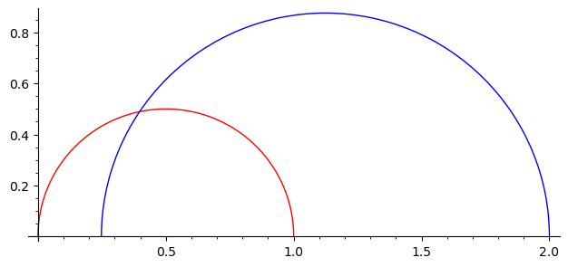
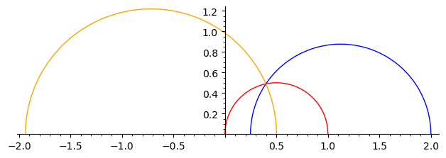
We plot some geodesics in the upper half plane and in the Klein model.
g = H.geodesic(0, 1)
h = H.geodesic(1/2 - a/5, 2)

g.plot(color="red") + h.plot(color="blue")
g.plot(model="klein", color="red") + h.plot(model="klein", color="blue")
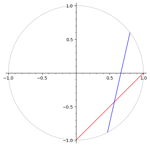
We determine the point of intersection of these geodesics. Note that that point has no coordinates in the upper half plane (without going to a quadratic extension).
P = g.intersection(h)
P.coordinates(model="klein")
(-480/15193*a^2 - 2000/15193*a + 11924/15193,
 -480/15193*a^2 - 2000/15193*a - 3269/15193)
P.change_ring(AA).coordinates(model="half_plane")
(0.3974561732377553?, 0.4893718050653866?)
We use that point to define another geodesic to the infinite point ½.
g.plot(color="red") + h.plot(color="blue") + H.geodesic(P, 1/2).plot(color="orange")
Further Reading#
the
module referencefor hyperbolic geometry
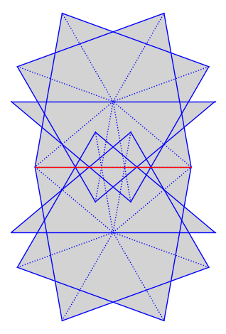
Veech Surfaces#
We can explore how a Veech surfaces decomposes into cylinders.
from flatsurf import polygons, similarity_surfaces, GL2ROrbitClosure

T = polygons.triangle(1, 4, 7)
S = similarity_surfaces.billiard(T).minimal_cover('translation')
S = S.erase_marked_points()

S.plot()
O = GL2ROrbitClosure(S)
decomposition = O.decomposition((1, 0))

decomposition
FlowDecomposition with 4 cylinders, 0 minimal components and 0 undetermined components
bool(decomposition.parabolic()) # the underlying value is a tribool, since it could be undetermined
True
Further Reading#
the
module referencerelated to the \(GL_2(\mathbb{R})\)-orbit closure
Strata & Orbit Closures#
We can query the stratum a surface belongs to, and then (often) determine whether the surface has dense orbit closure.
from flatsurf import similarity_surfaces, polygons

T = polygons.triangle(2, 3, 8)
S = similarity_surfaces.billiard(T).minimal_cover('translation')

S.stratum()
H_6(7, 2, 1)
from flatsurf import GL2ROrbitClosure

O = GL2ROrbitClosure(S)
O
GL(2,R)-orbit closure of dimension at least 2 in H_6(7, 2, 1) (ambient dimension 14)
for decomposition in O.decompositions(10, limit=20):
    if O.dimension() == O.ambient_stratum().dimension():
        break
    O.update_tangent_space_from_flow_decomposition(decomposition)

O
GL(2,R)-orbit closure of dimension at least 14 in H_6(7, 2, 1) (ambient dimension 14)
Further Reading#
the
module referencerelated to the \(GL_2(\mathbb{R})\)-orbit closure
Veering Triangulations#
We create a Veering triangulation from the stratum \(H_2(2)\).
from veerer import VeeringTriangulation, FlatVeeringTriangulation
from surface_dynamics import Stratum

H2 = Stratum([2], 1)
VT = VeeringTriangulation.from_stratum(H2)

VT
VeeringTriangulation("(0,6,~5)(1,8,~7)(2,7,~6)(3,~1,~8)(4,~2,~3)(5,~0,~4)", "RRRBBBBBB")
If you aim to study a specific surface, you might need to input the veering triangulation manually.
triangles = "(0,~7,6)(1,~5,~2)(2,4,~3)(3,8,~4)(5,7,~6)(~8,~1,~0)"
edge_slopes = "RBBRBRBRB"
VT2 = VeeringTriangulation(triangles, edge_slopes)

VT2
VeeringTriangulation("(0,~7,6)(1,~5,~2)(2,4,~3)(3,8,~4)(5,7,~6)(~8,~1,~0)", "RBBRBRBRB")
VT2.stratum()
/home/runner/work/sage-flatsurf/sage-flatsurf/.pixi/envs/doc/lib/python3.12/site-packages/surface_dynamics/flat_surfaces/abelian_strata.py:238: UserWarning: AbelianStratum has changed its arguments in order to handle meromorphic and higher-order differentials; use Stratum instead
  warnings.warn('AbelianStratum has changed its arguments in order to handle meromorphic and higher-order differentials; use Stratum instead')
H_2(2)
We play with flat structures on a Veering triangulation. There are several pre-built constructions.
F0 = VT.flat_structure_middle()
F0.plot()
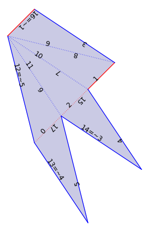
F1 = VT.flat_structure_geometric_middle()
F1.plot()
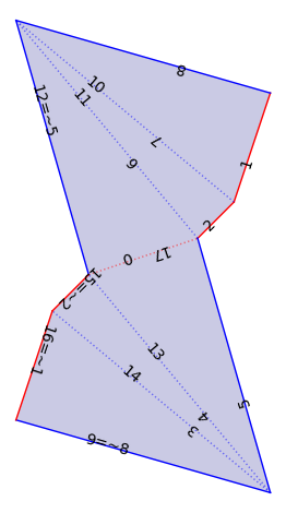
F2 = VT.flat_structure_min()
F2.plot()
We can work with \(L^{\infty}\)-Delaunay flat structures. These are also called geometry flat structures in veerer.
We check that the Veering triangulation VT corresponds to an open cell of the \(L^\infty\)-Delaunay decomposition of \(H_2(2)\).
VT.is_geometric()
True
We compute the cone of \(L^\infty\)-Delaunay data for the given Veering triangulation VT.
Each point in the cone corresponds to a geometric flat structure given as \((x_0, \ldots, x_8, y_0, \ldots, y_8)\) where \((x_i, y_i)\) is the holonomy of the \(i\)-th edge.
The geometric structure is a polytope. Here the ambient dimension 18 corresponds to the fact that we have 9 edges (each edge has an \(x\) and a \(y\) coordinate). The dimension 8 is the real dimension of the stratum (\(\dim_\mathbb{C} H_2(2) = 4\)).
geometric_structures = VT.geometric_polytope()

geometric_structures
Cone of dimension 8 in ambient dimension 18 made of 10 facets (backend=ppl)
The rays allow to build any vector in the cone via linear combination (with non-negative coefficients).
rays = list(map(QQ**18, geometric_structures.rays()))
If all entries are positive, we have a valid geometric structure on VT.
xy = rays[0] + rays[12] + rays[5] + 10 * rays[6] + rays[10] + rays[16]

xy
(13, 1, 1, 17, 16, 3, 16, 17, 18, 3, 3, 1, 25, 26, 29, 26, 25, 22)
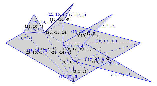
Construct the associated flat structure (note that x and y are inverted).
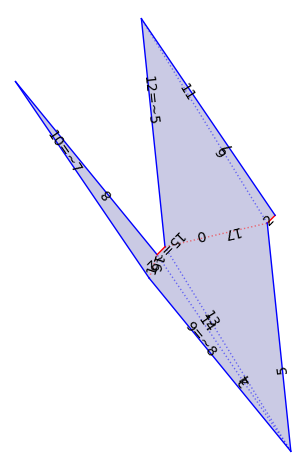
flat_veering = VT._flat_structure_from_train_track_lengths(xy[9:], xy[:9])

flat_veering.plot()
We now explore the \(L^\infty\)-Delaunay of a given linear family.
We do it for the ambient stratum, i.e., the tangent space is everything.
The object one needs to start from is a pair of a Veering triangulation and a linear subspace.
L = VT.as_linear_family()
The geometric automaton is the set of such pairs that one obtains by moving around in the moduli space.
Initially, there is only the pair we provided.
A = L.geometric_automaton(run=False)

A
Partial geometric veering linear constraint automaton with 1 vertex
A.run(10)

A
Partial geometric veering linear constraint automaton with 11 vertices
We could compute everything (until there is nothing more to be explored).
If the computation terminates, it proves that L was indeed the tangent space to a \(GL_2(\mathbb{R})\)-orbit closure.