Exploring Orbit Closures

We demonstrate how to use sage-flatsurf to compute the GL(2,R)-orbit closure of a surface. This example was interesting to P. Apisa and A. Wright.

Parts of this rely on the C++ library libflatsurf. Please consult our installation guide if it is not available on your system yet.

Building the Surface and Orbit Closure

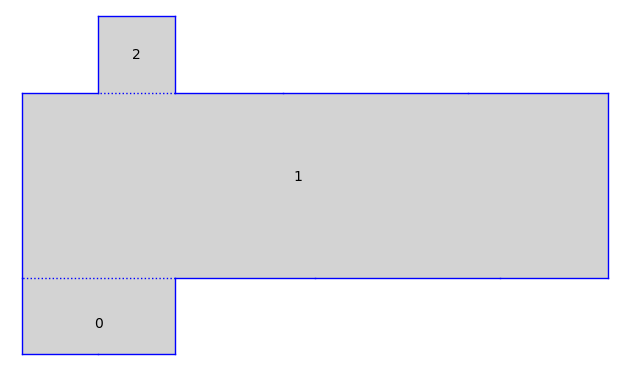
We consider the following half-translation surface

+---5---+
|       |
4       4
|       |
+       +---5---+---6---+---7---+---8---+
|                                       |
3                                       3
|                                       |
+               +---8---+---7---+---6---+
|               |
2               2
|               |
+---1---+---1---+

It belongs to \(Q_3(10, -1^2)\).

from flatsurf import Polygon, MutableOrientedSimilaritySurface


def apisa_wright_surface(h24, h3, l15, l6, l7, l8):
    K = Sequence([h24, h3, l15, l6, l7, l8]).universe().fraction_field()

    v24 = vector(K, (0, h24))
    v3 = vector(K, (0, h3))
    v15 = vector(K, (l15, 0))
    v6 = vector(K, (l6, 0))
    v7 = vector(K, (l7, 0))
    v8 = vector(K, (l8, 0))

    S = MutableOrientedSimilaritySurface(K)

    S.add_polygon(Polygon(edges=[v15, v15, v24, -2 * v15, -v24]))
    S.add_polygon(
        Polygon(edges=[2 * v15, v8, v7, v6, v3, -v8, -v7, -v6, -v15, -v15, -v3])
    )
    S.add_polygon(Polygon(edges=[v15, v24, -v15, -v24], base_ring=K))

    S.glue((0, 0), (0, 1))
    S.glue((0, 2), (0, 4))
    S.glue((0, 3), (1, 0))
    S.glue((1, 1), (1, 5))
    S.glue((1, 2), (1, 6))
    S.glue((1, 3), (1, 7))
    S.glue((1, 4), (1, 10))
    S.glue((1, 8), (2, 2))
    S.glue((1, 9), (2, 0))
    S.glue((2, 1), (2, 3))
    S.set_immutable()
    return S

We use some simple parameters:

K = QuadraticField(2)
a = K.gen()
S = apisa_wright_surface(1, 1 + a, 1, a, 1 + a, 2 * a - 1)
S.plot(edge_labels=False)

S

Half-Translation Surface in Q_3(10, -1^2) built from a square and 2 rectangles

Now build the canonical double cover and orbit closure:

U = S.minimal_cover("translation")
U.stratum()

H_6(5^2, 0^2)

Now build the orbit closure. The snippet below explores saddle connection up to length 16 looking for cylinders. Each decomposition into cylinders and minimal components provides a new tangent direction in the GL(2,R)-orbit closure of the surface via A. Wright’s cylinder deformation.

from flatsurf import GL2ROrbitClosure  # optional: pyflatsurf

O = GL2ROrbitClosure(U)  # optional: pyflatsurf
O.dimension()  # optional: pyflatsurf

/usr/share/miniconda3/envs/test/lib/python3.10/site-packages/cppyy/__init__.py:319: DeprecationWarning: pkg_resources is deprecated as an API. See https://setuptools.pypa.io/en/latest/pkg_resources.html
  import pkg_resources as pr

2

The above dimension is just the current dimension. At initialization it only consists of the GL(2,R)-direction.

old_dim = O.dimension()  # optional: pyflatsurf
for i, dec in enumerate(O.decompositions(16, bfs=True)):  # optional: pyflatsurf
    O.update_tangent_space_from_flow_decomposition(dec)
    new_dim = O.dimension()
    if old_dim != new_dim:
        holonomies = [cyl.circumferenceHolonomy() for cyl in dec.cylinders()]
        # .area() as reported by liblatsurf is actually twice the area
        areas = [cyl.area() / 2 for cyl in dec.cylinders()]
        moduli = [
            (v.x() * v.x() + v.y() * v.y()) / area for v, area in zip(holonomies, areas)
        ]
        u = dec.vertical().vertical()
        print("saddle connection number", i)
        print("holonomy           :", u)
        print("length             :", RDF(u.x() * u.x() + u.y() * u.y()).sqrt())
        print("num cylinders      :", len(dec.cylinders()))
        print("num minimal comps. :", len(dec.minimalComponents()))
        print("current dimension  :", new_dim)
        print("cyls. holonomies   :", holonomies)
        print("cyls. moduli       :", moduli)
        if new_dim == 7:
            break
        old_dim = new_dim
        print("-" * 30)

saddle connection number 0
holonomy           : (0, -1)
length             : 1.0
num cylinders      : 2
num minimal comps. : 2
current dimension  : 3
cyls. holonomies   : [(0, (-2*a-5 ~ -7.8284271)), (0, (-2*a-5 ~ -7.8284271))]
cyls. moduli       : [(2*a+5 ~ 7.8284271), (2*a+5 ~ 7.8284271)]
------------------------------
saddle connection number 1
holonomy           : (-1, 0)
length             : 1.0
num cylinders      : 6
num minimal comps. : 0
current dimension  : 4
cyls. holonomies   : [(-1, 0), (-2, 0), (-1, 0), (-2, 0), ((-4*a-2 ~ -7.6568542), 0), ((-4*a-2 ~ -7.6568542), 0)]
cyls. moduli       : [1, 2, 1, 2, (-2*a+6 ~ 3.1715729), (-2*a+6 ~ 3.1715729)]
------------------------------
saddle connection number 3
holonomy           : (-1, -1)
length             : 1.4142135623730951
num cylinders      : 2
num minimal comps. : 2
current dimension  : 5
cyls. holonomies   : [((-3*a-3 ~ -7.2426407), (-3*a-3 ~ -7.2426407)), ((-3*a-3 ~ -7.2426407), (-3*a-3 ~ -7.2426407))]
cyls. moduli       : [(12*a+18 ~ 34.970563), (12*a+18 ~ 34.970563)]
------------------------------

saddle connection number 9
holonomy           : (3, 1)
length             : 3.1622776601683795
num cylinders      : 2
num minimal comps. : 1
current dimension  : 6
cyls. holonomies   : [((3*a+3 ~ 7.2426407), (a+1 ~ 2.4142136)), ((3*a+3 ~ 7.2426407), (a+1 ~ 2.4142136))]
cyls. moduli       : [10, 10]
------------------------------

saddle connection number 88
holonomy           : ((-6*a+1 ~ -7.4852814), (5*a+7 ~ 14.071068))
length             : 15.938142508386589
num cylinders      : 2
num minimal comps. : 1
current dimension  : 7
cyls. holonomies   : [((-284*a ~ -401.63665), (268*a+376 ~ 755.00923)), ((-284*a ~ -401.63665), (268*a+376 ~ 755.00923))]
cyls. moduli       : [(47880*a+67904 ~ 135616.55), (47880*a+67904 ~ 135616.55)]