Graphics Configuration

Rearranging Polygons

from flatsurf.geometry.polyhedra import platonic_dodecahedron

s = platonic_dodecahedron()[1]

The default plot of this surface:

s.plot()

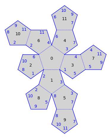
Labels in the center of each polygon indicate the label of the polygon. Edge labels above indicate which polygon the edge is glued to.

Plotting the surface is controlled by a GraphicalSurface object:

gs = s.graphical_surface()

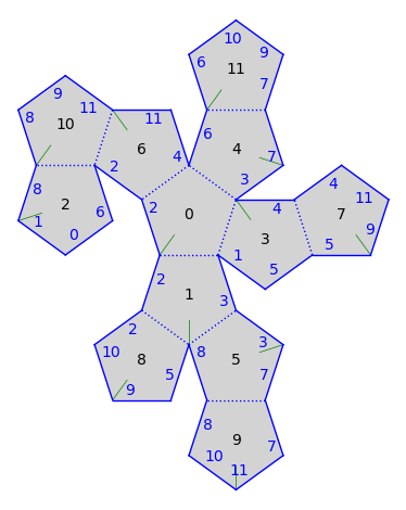
The graphical surface controls where polygons are drawn. You can glue a polygon across an edge using gs.make_adjacent(label, edge). A difficulty is that you need to know which edge is which. You can enable zero_flags to see the zero vertex of each polygon.

gs.will_plot_zero_flags = True

gs.plot()

sage-flatsurf uses a simple algorithm to layout polygons. Sometimes polygons overlap. But in this example the main concern is maybe that the picture is not as symmetric as we would like it to be. For example, we could aim for things to be symmetric around the polygons 0 and 1. Let’s say we would like to move polygon 2 so that it’s glued to 10 instead of being glued to 0. We count the edges on polygon 10 until we reach the edge glued to 2. It’s the first one. We can verify that this is correct:

s.opposite_edge(10, 0)

(2, 3)

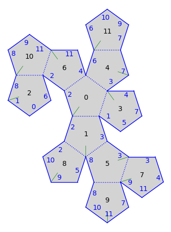
We can move polygon 2 so that it is adjacent to polygon 10 with the command:

gs.make_adjacent(10, 0)

Lets check that it worked:

gs.plot()

Let’s build the symmetric widget at polygon 1 by moving 7 to be adjacent to 5 and 3 to be adjacent to 7. Note that the order of the movements matter. If we do it in the wrong order, we detach things:

gs.make_adjacent(7, 3)
gs.make_adjacent(5, 4)
gs.plot()

Indeed, we moved 3 to be adjacent to 7 but then moved 7 away. Let’s do it in the correct order:

gs.make_adjacent(5, 4)
gs.make_adjacent(7, 3)
gs.plot()

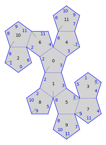
Finally, glue 9 to 8 for a symmetric picture:

gs.make_adjacent(8, 0)
gs.plot()

Moving between coordinate systems

The Euclidean Cone Surface s works in a different coordinate system then the graphical surface gs. So, when we moved the polygon above, we had no affect on s. In fact, the polygons of s are all the same:

s.polygon(0)

Polygon(vertices=[(0, 0), (2, 0), (-a^2 + 4, a^3 - 3*a), (1, a^3 - 4*a), (a^2 - 2, a^3 - 3*a)])

s.polygon(1)

Polygon(vertices=[(0, 0), (2, 0), (-a^2 + 4, a^3 - 3*a), (1, a^3 - 4*a), (a^2 - 2, a^3 - 3*a)])

So really s is a disjoint union of twelve copies of a standard pentagon with some edge gluings.

Lets now look at “graphical coordinates” i.e., the coordinates in which gs works.

show(gs.plot(), axes=True)

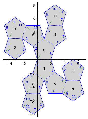
We can tell that the point (4, -4) is in the unfolding, but we can’t immediately tell if it is in polygon 5 or 7. The GraphicalSurface gs is made out of GraphicalPolygons which we can use to deal with this sort of thing.

gs.graphical_polygon(5).contains((4, -4))

False

gs.graphical_polygon(7).contains((4, -4))

True

Great. Now we can get the position of the point on the surface!

gp = gs.graphical_polygon(7)
pt = gp.transform_back((4, -4))
pt

(a^2 - 2*a - 4, a^3 + 2*a^2 - 5*a - 6)

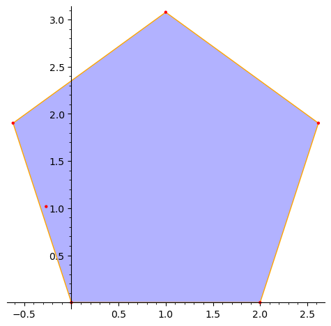
Here we plot polygon 7 in its geometric coordinates with pt.

s.polygon(7).plot() + point2d([pt], zorder=100, color="red")

Lets convert it to a surface point and plot it!

Note that we will have to pass the graphical surface to the point so it plots with respect to gs and not with respect to s.graphical_surface.

spt = s.point(7, pt)
spt

Point (a^2 - 2*a - 4, a^3 + 2*a^2 - 5*a - 6) of polygon 7

gs.plot() + spt.plot(gs, color="red", size=20)

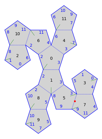
Now we want to plot an upward trajectory through this point. Again, we have to deal with the fact that the coordinates might not match. You can get access to the transformation (a similarity) from geometric coordinates to graphical coordinates:

transformation = gs.graphical_polygon(7).transformation()
transformation

(x, y) |-> ((-1/2*a^2 + 3/2)*x + (-1/2*a)*y + (-a^2 + 5), (1/2*a)*x + (-1/2*a^2 + 3/2)*y + (-2*a^3 + 7*a))

Really we want the inverse:

inverse_transformation = ~transformation
inverse_transformation

(x, y) |-> ((-1/2*a^2 + 3/2)*x + (1/2*a)*y + (3*a^2 - 10), (-1/2*a)*x + (-1/2*a^2 + 3/2)*y + (a^3 - 3*a))

We just want the derivative of this similarity to transform the vertical direction. The derivative is a \(2 \times 2\) matrix.

show(inverse_transformation.derivative())

\(\displaystyle \left(\begin{array}{rr} -\frac{1}{2} a^{2} + \frac{3}{2} & \frac{1}{2} a \\ -\frac{1}{2} a & -\frac{1}{2} a^{2} + \frac{3}{2} \end{array}\right)\)

direction = inverse_transformation.derivative() * vector((0, 1))
direction

(1/2*a, -1/2*a^2 + 3/2)

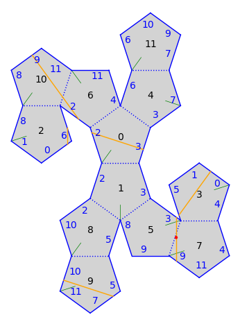
We can use the point and the direction to get a tangent vector, which we convert to a trajectory, flow and plot.

tangent_vector = s.tangent_vector(7, pt, direction)
tangent_vector

SimilaritySurfaceTangentVector in polygon 7 based at (a^2 - 2*a - 4, a^3 + 2*a^2 - 5*a - 6) with vector (1/2*a, -1/2*a^2 + 3/2)

traj = tangent_vector.straight_line_trajectory()
traj.flow(100)
traj.is_closed()

True

gs.plot() + spt.plot(gs, color="red") + traj.plot(gs, color="orange")

Multiple graphical surfaces

It is possible to have more than one graphical surface. Maybe you want to have one where things look better. To get a new suface, you can call s.graphical_surface() again.

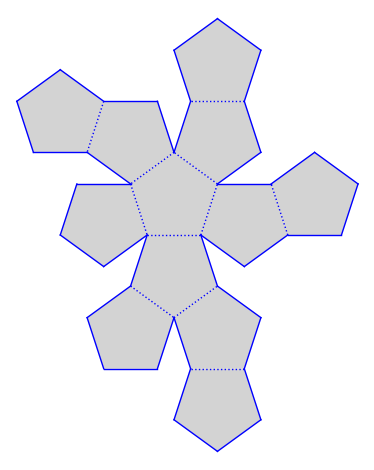
pretty_gs = s.graphical_surface(polygon_labels=False, edge_labels=False)

pretty_gs.plot()

Current polygon printing options:

pretty_gs.polygon_options

{'color': 'lightgray'}

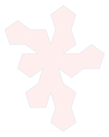
del pretty_gs.polygon_options["color"]
pretty_gs.polygon_options["rgbcolor"] = "#ffeeee"

pretty_gs.non_adjacent_edge_options["thickness"] = 0.5
pretty_gs.non_adjacent_edge_options["color"] = "lightblue"
pretty_gs.will_plot_adjacent_edges = False

pretty_gs.plot()

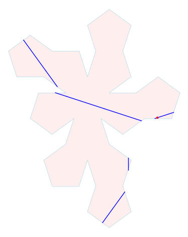
Again, to use a non-default graphical surface, we need to pass the graphical surface as a parameter.

pretty_gs.plot() + spt.plot(pretty_gs, color="red") + traj.plot(pretty_gs)

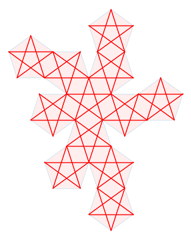
Lets make it prettier by drawing some stars on the faces!

Find all saddle connections of length at most \(\sqrt{16}\):

saddle_connections = s.saddle_connections(16)

The edges have length two so we will keep anything that has a different length.

saddle_connections2 = []
for sc in saddle_connections:
    h = sc.holonomy()
    if h[0] ** 2 + h[1] ** 2 != 4:
        saddle_connections2.append(sc)
len(saddle_connections2)

120

plot = pretty_gs.plot()
for sc in saddle_connections2:
    plot += sc.plot(pretty_gs, color="red")
plot

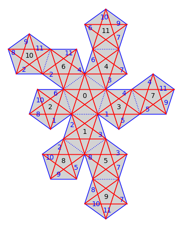
Plot using the original graphical surface.

plot = s.plot()
for sc in saddle_connections2:
    plot += sc.plot(color="red")
plot

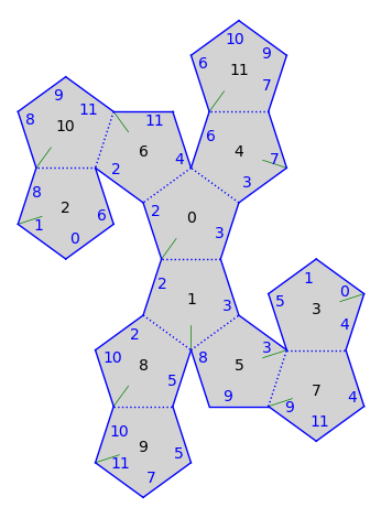
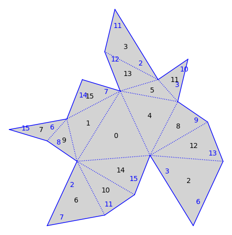
Manipulating edge labels

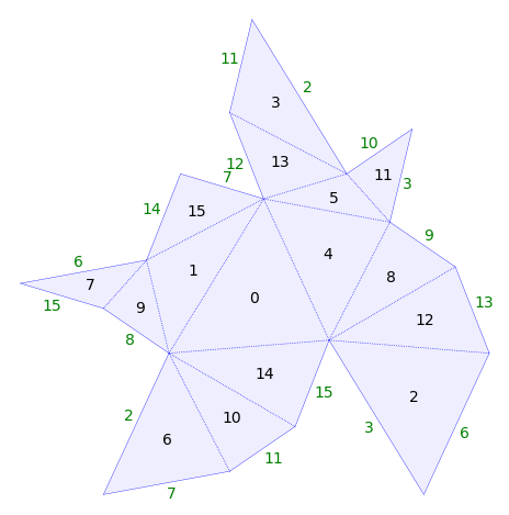
from flatsurf import translation_surfaces

s = translation_surfaces.arnoux_yoccoz(4)

s.plot()

Here is an example with the edge labels centered on the edge.

gs = s.graphical_surface(cached=False)

/usr/share/miniconda3/envs/test/lib/python3.10/site-packages/flatsurf/geometry/categories/euclidean_polygonal_surfaces.py:104: UserWarning: The cached keyword has been removed from graphical_surface(). The keyword is ignored in this version of sage-flatsurf and will be dropped completely in a future version of sage-flatsurf. The result of graphical_surface() is never cached anymore.
  warnings.warn(

del gs.polygon_options["color"]
gs.polygon_options["rgbcolor"] = "#eee"
gs.edge_label_options["position"] = "edge"
gs.edge_label_options["t"] = 0.5
gs.edge_label_options["push_off"] = 0
gs.edge_label_options["color"] = "green"
gs.adjacent_edge_options["thickness"] = 0.5
gs.will_plot_non_adjacent_edges = False

gs.plot()

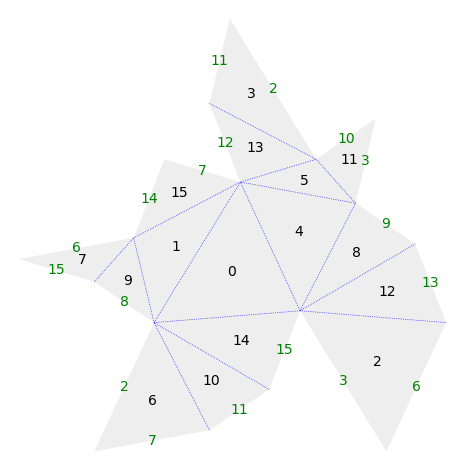
gs = s.graphical_surface(cached=False)

del gs.polygon_options["color"]
gs.polygon_options["rgbcolor"] = "#eef"
gs.edge_label_options["position"] = "outside"
gs.edge_label_options["t"] = 0.5
gs.edge_label_options["push_off"] = 0.02
gs.edge_label_options["color"] = "green"
gs.adjacent_edge_options["thickness"] = 0.5
gs.non_adjacent_edge_options["thickness"] = 0.25

gs.plot()